In 2018, Two transformer models were released that combined self-attention with transfer learning capabilities, opening the floodgate of using Transformers in NLP and propelled introduction of subsequent language models:

• GPT: “Improving language understanding by generative pre-training” (Radford et al. 2018). Uses decoder part of Transformer to predict words in an autoregressive manner.
• BERT: “BERT: pre-training of deep bidirectional transformers for language understanding” (Devlin et al. 2018). Uses encoder part of Transformer and performs masked language modeling (MLM). These models open the floodgate of using Transformers in NLP and propelled introduction of subsequent language models. This article describes the Transformer architecture.

You can regard the Transformer as a “sequence to sequence” model. Given a set of input embedding vectors $\mathbf{x} = [x_1, \ldots, x_N]$, perform a sequence of layer transformations to produce as output, contextualized embeddings $\mathbf{y} = [y_1, \ldots, y_N]$.

Some notes on the Transformer architecture:

• The Transformer is highly efficient, as it allows parallel computations of the individual output vectors $y_i$.
• It has perfect long-term memory, because part of the process in producing each $y_i$ is a weighted sum over all the inputs (time steps) in the sequence. However, also due to this, self-attention is quadratic in computation cost.
• Note that each individual output $y_i$ from a single self-attention layer is aggregated from “pairs of inputs”. In practical Transformer architectures, we stack multiple Transformer blocks. This allows us to aggregate information from “pairs of pairs”, and so on.
• Fundamentally, the self-attention is a set-to-set layer, with no access to the sequential structure of the inputs. Thus, we encode the position index of each input as position embeddings. This is aggregated with the input embedding vectors, to serve as input to the rest of the Transformer block.
• The Transfomer leverages two techniques that are crucial towards building very deep networks: skipped connections (a.ka. residual connections), and layer normalization.
• The layer normalization layers and feed forward layer are applied on each individual embedding (time step)

Transformer Overview

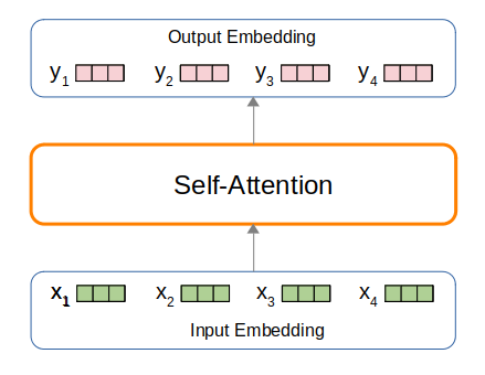
At the core of the Transforrmer architecture is the self-attention mechanism. Given a sequence of input tokens $\mathbf{t} = [t_1, \ldots, t_i, \ldots, t_N]$, the Transformer first represent each $t_i$ by an embedding vector $x_i$ (a list of floating point numbers). The self attention mechanism then produces as output a sequence $\mathbf{y} = [y_1, \ldots, y_i, \ldots, y_N]$.

• Each $y_i$ is a contextualized embedding vector, where “contextualized” means that $y_i$ is derived by performing a weighted sum over the entire sequence: $y_i = \sum_{j} w_{ij} x_j$.
• Here, $w_{ij}$ represents the affinity or similarity between $x_i$ and $x_j$ and is calculated by performing softmax over dot-products: $w_{ij} = \frac{\text{exp}(x_i^T x_j)}{\sum_j \text{exp}(x_i^T x_j)}$
• Intuitively, the weighted sum is a selective summary of the information contained in all the tokens of the sequence, giving as output a fixed sized representation $y_i$ of an arbitrary set of inputs ${x_i}$, for $1 \le i \le N$.

We now describe the Transformer architecture in more details. We start by diving into the self-attention mechanism, then describe multi-head attention, and finally bring all these together via a Transformer block.

Single-Head Attention

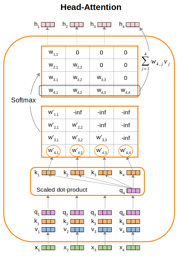
We assume that the sequence of input tokens is represented by a corresponding sequence of input embeddings $\textbf{x} = [x_1, \ldots, x_j, \ldots, x_N]$. We illustrate a “single-head” self-attention mechanism in the following Figure (we describe multi-head in the next Section) by using an example of 4 embedding vectors $x_1$ to $x_4$.

Query, Key, and Value

Note that each input embedding $x_i$ plays three different roles (used in 3 different places). Specifically, recall from the above Overview Section, we mentioned that $y_i = \sum_{j} w_{i,j} x_j$:

• We first calculate dot products: $w_{ij} = \text{softmax}(x_i^T x_j)$. We refer to the $x_i$ here as “query” and $x_j$ as “key”.
• Then, we calculate $y_i = \sum_{j} w_{ij} x_j$. We refer to the $x_j$ here as “value”.

To allow learnable parameterization, we introduce parameter matrices $Q$ (query), $K$ (key), and $V$ (value), which are represented as linear layers, to project each $x_i$ into $q_i$, $k_i$, and $v_i$: * $q_i = Q x_i$ * $k_i = K x_i$ * $v_i = V x_i$

Affinity Scores and Weighted Sum

Next, we calculate dot-products between the query vectors and key vectors as a measure of affinity scores.

• As an example, $w^{‘}_{4,1} = q_4 \cdot k_1$ represents the affinity of $x_4$ with $x_1$.
• Referring to the above Figure, performing dot-products using $q_4$ give us a list of $w^{‘}_{4,j}$ for $1 \le j \le 4$, which represents the affinity of $x_4$ with $x_1, x_2, x_3$, and $x_4$ respectively.

Once we have the dot-product score matrix $W^{‘}$, we apply softmax on each individual row to obtain the $W$ softmax weight matrix. We then perform a weighted sum over the value embeddings to produce the hidden output representations of the attention layer, e.g. $h_4 = \sum_{j} w_{4,j} v_j$.

Scaled Dot Product

Note that the Figure we provide mentions “scaled” dot-product, instead of plain dot-product.

• As the dimensionality of the $x$ embedding vectors grows, so does the average scale of the dot-product values $w^{‘}$, thereby increasing the variance of $w^{‘}$. This means that some particular $w^{‘}_{ij}$ might be particularly large in relation to the other scores $w^{‘}$.
• Recall that in the weighted sum $y_i = \sum_{j} w_{ij} x_j$, the weight $w_{ij}$ is a softmax over the dot-product score $w^{‘}_{ij}$. When the variance of the inputs $w^{‘}$ increases, the resultant softmax might get very “peaky” on a single $w^{‘}$, thereby restricting the weighted sum to just focusing on a single $x_j$. To mitigate this, the authors of the self-attention paper use scaled dot product in self-attention: $\frac{x_i^T x_j}{\sqrt{K}}$, where $K$ is the length (dimensionality) of vector $x$.
• To understand why we scale by a function of $K$, recall that in statistics, if $X$ and $Y$ are two independent random variables, then:
  • $\text{Var}(XY) = (\text{Var}(X) + \mathbb{E}[X]^2) (\text{Var}(Y) + \mathbb{E}[Y]^2) - \mathbb{E}[X]^2 \mathbb{E}[Y]^2$
• Then, given a pair of vectors $x_i$ and $x_j$ (both having $K$ dimensions or components) where each vector component is independent from one another, and follows a distribution with 0 mean and 1 variance.
  • The variance of a particular component pair is: \(\text{Var}(x_i^k, x_j^k) = (\text{Var}(x_i^k) + \mathbb{E}[x_i^k]^2) (\text{Var}(x_j^k) + \mathbb{E}[x_j^k]^2) - \mathbb{E}[x_i^k]^2 \mathbb{E}[x_j^k]^2 = 1\)
  • Thus the variance of the dot-product $\text{Var}(\sum_{k=0}^{K} x_i^k x_j^k) = \sum_{k=0}^{K} \text{Var}(x_i^k, x_j^k) = K$

Normalization helps to ensure better stability during training. For instance, if our pre-activations values are large (either very negative or very positive), passing along these values to an activation function such as tanh will result in output values that are close to -1 or +1, which are regions with very low gradients (and thus inefficient backpropagation).

Auto-Regressive Masking

Notice also that in the Figure, we are masking out scores in the upper triangular. This is suitable for autoregressive language models like GPT, which are trained to predict the next word given past contexts. In this setting, we have to mask future connections to prevent the model from “looking ahead” during training to trivially predict the next token. Specifically, we apply a mask in the upper triangular by setting $w^{‘}_{ij} = -\infty$ if $j \gt i$. After applying softmax (which applies exponential first followed by normalization), the upper triangular becomes zeros, since $\text{exp}(-\infty) = 0$.

Self Attention Code for a Single Head

The self-attention layer could be implemented as follows:

class HeadAttention(nn.Module):
    def __init__(self, head_size):
        super().__init__()
        self.query = nn.Linear(embed_size, head_size, bias=False)
        self.key = nn.Linear(embed_size, head_size, bias=False)
        self.value = nn.Linear(embed_size, head_size, bias=False)
        self.head_size = head_size        
        self.register_buffer('attmask', torch.tril(torch.ones(block_size, block_size)))
        self.dropout = nn.Dropout(dropout)

    def forward(self, x):
        batch_size, seq_len, embed_size = x.shape
        q = self.query(x)
        k = self.key(x)        
        v = self.value(x)
		
        # compute attention scores
        normalizer = self.head_size**-0.5
        weights = q @ k.transpose(-2, -1) * normalizer
		     
        # weights.shape = (batch_size, seq_len, seq_len)
        weights = weights.masked_fill(self.attmask[:T, :T] == 0, float('-inf'))    
        weights = F.softmax(weights, dim=-1) # softmax along last dimension
        weights = self.dropout(weights)
		
        # perform the weighted aggregation of the values        
        # (batch_size, seq_len, seq_len) @ (batch_size, seq_len, embed_size) 
        # -> (batch_size, seq_len, embed_size)
        output = weights @ v  		
        return out

Notes:

• The code snippet weights = q @ k.transpose(-2, -1) * normalizer corresponds to scaled dot-products.
• PyTorch buffers are named tensors that do not update gradients at every step, unlike parameters which are trainable. But buffers will be saved as part of state_dict, moved to cuda() or cpu() with the rest of the model’s parameters, cast to float/double with the rest of the model’s parameters.
• The code snippet weights.masked_fill(.) enables auto-regressive masking. This is suitable for decoder style language models. If we are building an encoder style Transformer that considers both past and future contexts, we simply comment out the the weights.masked_fill(.) line of code.

Multi-Head Attention

Given a sentence such as “This movie was not too bad”, you can see that there are various word-pair relations:

• “bad” is a property of the “movie”
• “not” inverts the sentiment “bad”
• “too” moderates the word “bad”

A piece of text will contain many different phenomenon. Asking a single self-attention module to model all these different relations between words might be too difficult. Thus in practice, we perform multi-head attention which employs multiple self-attention modules to generate their own hidden representations, and then subsequently combine these representations. We illustrate multi-head attention using the Figure below.

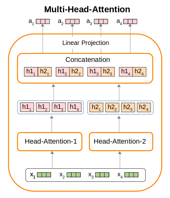
In the Figure above, we illustrate a multi-head attention module that employs two individual self-attention modules. Given input embeddings $\mathbf{x} = [x_1, x_2, x_3, x_4]$, the first self-attention module produces hidden representations $h1_1$ to $h1_4$, while the second self-attention module produces $h2_1$ to $h2_4$. Thereafter, we concatenate $(h1_i, h2_i)$, for $1 \le i \le 4$, perform linear projections on each individual concatenated result, to produce output vectors $a_i$.

The multi-head attention layer could be implemented as follows:

class MultiHeadAttention(nn.Module):
    def __init__(self, num_heads, head_size):
        super().__init__()
        self.heads = nn.ModuleList(HeadAttention(head_size) for _ in range(num_heads))
        self.proj = nn.Linear(embed_size, embed_size)
        self.dropout = nn.Dropout(dropout)

    def forward(self, x):
        # x.shape = (batch_size, seq_len, embed_size)
        # concat along the last dimension, i.e. the embed_size
        out = torch.cat([h(x) for h in self.heads], dim=-1)  
        out = self.dropout(self.proj(out))
        return out

Transformer Block

We are now ready to put everything together in a Transformer block, which we illustrate in the following Figure.

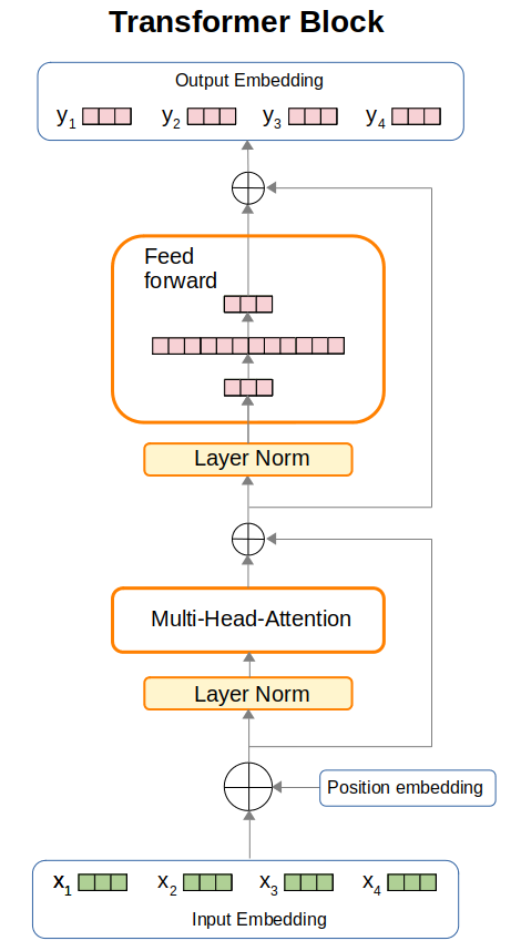
We now describe the flow of inputs to outputs in the Transformer block:

• Given an input tokenized text sequence, we first convert each token to its integer index in the vocabulary, producing idx (a list of integers). We use idx to index into the embedding table, encode the positions using a separate position embedding table, then aggregate them to produce the inputs to the first layer normalization layer. A sample code snippet could be as follows:

    self.token_embedding_table = nn.Embedding(vocab_size, embed_size)
    self.position_embedding_table = nn.Embedding(seq_len, embed_size)
    ...
    def forward(self, idx):
        batch_size, seq_len = idx.shape
        input_emb = self.token_embedding_table(idx)
        pos_emb = self.position_embedding_table(torch.arange(seq_len, device=device))
        x = input_emb + pos_emb
  

• The inputs are then passed through a layer normalization layer, followed by a multi-head attention layer. The outputs are then aggregated with a skipped connection (a.k.a. residual connection). A sample code snippet is as follows:

    def __init__(self, embed_size, no_of_heads):
        head_size = embed_size // no_of_heads
        self.layer_norm1 = nn.LayerNorm(embed_size)
        self.multihead_att = MultiHeadAttention(n_head, head_size)
  	      
    def forward(self, x):
        x = self.layer_norm1(x)
        x = x + self.multihead_att(x)
  

• The aggregated representations are then passed through a second layer normalization layer, followed by a feed forward layer. The outputs are then aggregated with a skipped connection, to produce the final output embeddings of this Transformer block.

A sample code snippet for the Transformer block is as follows:

class FeedForward(nn.Module):
    def __init__(self, embed_size):
        super().__init__()
        self.network = nn.Sequential(
            nn.Linear(embed_size, 4 * embed_size),
            nn.ReLU(),
            nn.Linear(4 * embed_size, embed_size),
            nn.Dropout(dropout)
        )

    def forward(self, x):
        return self.network(x)

class TransformerBlock(nn.Module):
    def __init__(self, embed_size, n_head):
        super().__init__()
        head_size = embed_size // n_head
        self.multihead_att = MultiHeadAttention(n_head, head_size)
        self.ffwd = FeedForward(embed_size)
        self.layer_norm1 = nn.LayerNorm(embed_size)  
        self.layer_norm2 = nn.LayerNorm(embed_size)

    def forward(self, x):
        # x.shape = (batch_size, seq_len, embed_size)
        x = x + self.multihead_att(self.layer_norm1(x))
        x = x + self.ffwd(self.layer_norm2(x))
        return x

Some notes:

• PyTorch nn.Sequential vs nn.ModuleList:
  • In the above code, we used an object of type nn.Sequential. This has a forward() method. When defining blocks within nn.Sequential, we must be careful to ensure that the output size of a block matches the input size of the following block.
  • On the other hand, nn.ModuleList does not have a forward() method, i.e. there is no connection between each of the nn.Module that it stores. The advantage of using nn.ModuleList instead of using conventional Python lists to store modules, is that Pytorch is “aware” of the existence of the modules within an nn.ModuleList.