To train deep neural networks, we require techniques to stabilize training and reduce problems such as vanishing gradients. In this article, we discuss Skipped Connection and Layer Normalization.

Skipped Connection

One important technique that enables building very deep neural networks is Skipped connection (a.k.a residual connection). Consider that at layer $l+1$, activation result $a$ is defined as: $a^{l+1} = g(z^{l+1} + a^l)$, where $g$ denotes an activation function and $z^{l+1}$ denotes weights of layer $l+1$. By setting $z^{l+1}$ to 0, then $a^{l+1} = a^l$. This serves as a baseline and provides opportunity for the learned network (which also uses $z^{l+1}$) to be better than this baseline. The Figure below illustrates skipped connection being used as part of a network.

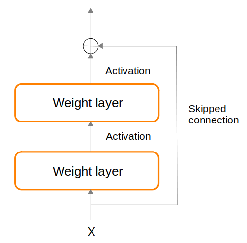
The skipped connection represents a baseline pathway that the network could use. But the network is also free to fork off and perform additional computations using the weights layers, and then projecting that result back onto the skipped connection pathway via addition.

During backpropagation, the gradients from the loss is allowed to flow equally between the skipped connection pathway and the alternative computation branch of weights layers, helping to reduce the problem of vanishing gradient. At the onset of training, the alternative computation branch might contribute little towards the network, but could gradually contribute more as training progresses.

Layer Normalization

Given a batch $b$ containing multiple input vectors (one per time-step $t$), we normalize each input vector $x^{bt}$ individually, to produce output vector $y^{bt}$ with mean 0 and standard deviation 1:

• We define $d$ as the dimensionality of $x^{bt}$, $i$ as an index into the individual dimension (or component) of $x^{bt}$. We also define $\gamma$ and $\beta$ as network learnable parameters. We then calculate the following.
• $\mu^{bt} = \frac{1}{d} \sum_{i} x_i^{bt}$ : (mean of the input vector)
• $\sigma^{bt} = \frac{1}{d} \sum_{i} (x_i^{bt} - \mu^{bt})^2$ : (variance of the input vector)
• $\hat{x}^{bt} = \frac{x^{bt} - \mu^{bt}}{\sqrt{\sigma^{bt}} + \epsilon}$ : (standarize, and $\epsilon$ for numerical stability)
• $y^{bt} = \gamma^{T} \hat{x}^{bt} + \beta$ (rescaling)

Note that without the final rescaling, we will always be forcing the output $y^{bt}$ to have mean 0 and standard deviation 1 (standard Gaussian). However, we only want this distribution at the onset of training, and wish to allow the network the flexibility to move away from this initial distribution as training progresses. So, layer normalization also makes use of learnable parameters $\gamma$ and $\beta$.

The above normalizes each individual sample. There is another normalization called batch normalization, which normalizes each individual feature, i.e. calculate $\mu$ and $\sigma$ for each individual feature and then normalize.

Root Mean Square Layer Normalization (RMSNorm)

The success of LayerNorm is attributed to its re-centering and re-scaling. The RMSNorm paper hypothesize that the re-scaling is the reason for success of LayerNorm, rather than re-centering.

Hence, RMSNorm is proposed, which focuses only on re-scaling to normalize each individual sample $x$ with dimension $n$: \(\text{RMS}(\vec{x}) = \sqrt{\frac{1}{n} \sum\limits_{i=1}^{n} x_{i}^{2}}\)

RMSNorm simplifies LayerNorm by removing the mean statistic, thus saving computation time. Note that when the mean of summed inputs is zero, RMSNorm is exactly equal to LayerNorm.