An optimizer helps to update network parameters as training iterations proceed. Here we describe Gradient Descent (SGD), SGD with momentum, RMSProp, and Adam.

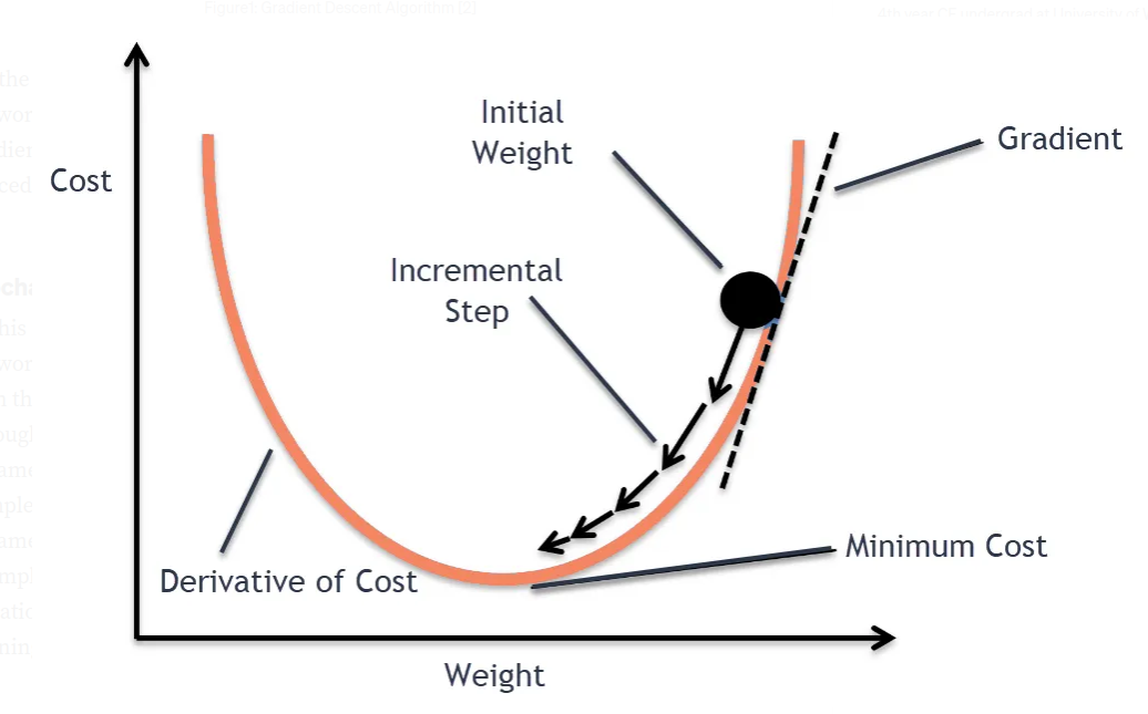
Gradient Descent

We compute the gradient of the cost function $J(\theta)$ w.r.t. the parameters $\theta$ for the entire training set: $\theta_{j} \leftarrow \theta_{j} - \alpha \frac{\partial}{\partial \theta_{j}} J(\theta)$

Exponentially Weighted Moving Average (EWA):

Let $V_{0} = 0$ and $\theta_{t}$ denote the parameter value at current time $t$. Then we compute the EWA $V_t$ as follows: \(V_{t} = \beta V_{t-1} + (1 - \beta) \theta_{t}\) In practice, we directly overwrite $V_t$, so we can also rewrite the above as follows: \(V_{t} = \beta V_{t} + (1 - \beta) \theta_{t}\)

$V_{t}$ is approximately averaging over $\frac{1}{1 - \beta}$ days of temperature. So if $\beta = 0.9$, then we are approximately averaging over 10 days of weights.

Bias correction: Since $V_t = 0$, for the initial few time periods, $V_t$ will be an under-estimate. We can perform bias correction for this by calculating $\frac{V_t}{1 - \beta^t}$:

• When $t$ becomes large, $1 - \beta^t$ becomes close to 1, and the bias correction will wear off.

SGD with Momentum

In essence, we compute exponentially weighted average of the gradient, and use that gradient to update the weights. This allows you to dampen out the oscillations in your gradients.

Initialize $V_{\partial \theta}=0$. Then on iteration $t$:

• Compute $\frac{\partial L}{\partial \theta}$ on current mini-batch as per normal
• Then compute $V_{\partial \theta} = \beta V_{\partial \theta} + (1 - \beta) \frac{\partial L}{\partial \theta}$. We normally set $\beta = 0.9$
• Now instead of doing $\theta = \theta - \alpha \frac{\partial L}{\partial \theta}$, we compute: $\theta = \theta - \alpha V_{\partial \theta}$

RMSProp

The main idea is to keep track of the moving average of the squared gradients for each weight. Then we use this to divide the gradient.

Set $S_{\partial \theta}=0$. On iteration t:

• Compute $\frac{\partial L}{\partial \theta}$ on current mini-batch as per normal
• $S_{\partial \theta} = \beta_2 S_{\partial \theta} + (1 - \beta_2) (\partial \theta)^2$ , usually set $\beta_2 = 0.999$
• $\theta = \theta - \alpha \frac{\partial \theta}{\sqrt{S_{\partial \theta}} + \epsilon}$

The above allows to self adapt the learning of the individual weights. For a particular weight $\theta_j$ that has a large gradient $\partial \theta_j$, then $S_{\partial \theta_j}$ will be large. Since we are dividing by a large number, then updates to $\theta_j$ will be small. Conversely, if the gradient of $\theta_i$ is small, then dividing by a small number, will cause us to make larger updates to $\theta_i$

Adam

This simply combines SGD with momentum, and RMSProp.

Initialize $V_{\partial \theta}=0$ and $S_{\partial \theta}=0$. On iteration $t$:

• Compute $\frac{\partial L}{\partial \theta}$ on current mini-batch as per normal
• SGD momentum: $V_{\partial \theta} = \beta_1 V_{\partial \theta} + (1 - \beta_1) \partial \theta$
• RMSProp: $S_{\partial \theta} = \beta_2 S_{\partial \theta} + (1 - \beta_2) (\partial \theta)^2$
• $\theta = \theta - \alpha \frac{V_{\partial \theta}}{\sqrt{S_{\partial \theta}} + \epsilon}$