
Linear Algebra
Here we will review the basis of linear algebra, which should help towards understand techniques such as Low Rank Adaptation (LoRA).
Basic Concepts
-
Span: The span of a set of vectors is the set of all possible linear combinations that can be formed by those vectors. E.g. the span of two vectors $\vec{v}$ and $\vec{w}$, is the set of all their linear combinations: $a \vec{v} + b \vec{w}$, where $a$ and $b$ are real number scalars.
-
Linear independence: If $\vec{u}$ is linearly independent from $\vec{v}$ and $\vec{w}$, then $\vec{u} \neq a \vec{v} + b \vec{w}$, for all scalar values of $a$ and $b$. Linear independence implies that no vector in a set can be expressed as a linear combination of the others. In other words, it’s the absence of redundancy in the set.
- Basis: A basis for a vector space is a set of vectors that:
- Spans the vector space, i.e. any vector in the vector space can be expressed as a linear combination of the basis vectors.
- Is linearly independent, i.e. no vector in the basis can be expressed as a linear combination of the other vectors. It’s the minimal set of vectors that can represent the entire space.
- A basis is not unique; different sets of vectors can serve as bases for the same vector space.
- Dimension: The dimension of a vector space is simply the number of vectors in a basis for that space.
Think of Matrics as Linear Transforms
Everytime you see a matrix, think of it as a certain transformation of space. Different matrices correspond to different transformations, such as rotations, scalings, and shears.
Assume that you have a 2 dimensional coordinate system with $\hat{i}$ and $\hat{j}$ defined as basis vectors. After you apply some linear transformation to the coordinate system, $\hat{i}$ lands at coordinates $[\hat{i}_1, \hat{i}_2]$, and $\hat{j}$ lands at coordinates $[\hat{j}_1, \hat{j}_2]$.
- In a linear transformation, grid lines remain parallel and evenly spaced, and the origin remains fixed.
-
Then given any general untransformed vector $[x, y]$, its coordinates after the same linear transform will be: \(x\begin{bmatrix}\hat{i}_1\\ \hat{i}_2 \end{bmatrix} + y\begin{bmatrix}\hat{j}_1\\ \hat{j}_2 \end{bmatrix}\)
-
It is common to capture linear transformations in the form of a matrix: \(\begin{bmatrix}\hat{i}_1 & \hat{j}_1\\ \hat{i}_2 & \hat{j}_2 \end{bmatrix}\)
-
Hence, the following matrix multiplication is just a way to compute what the transformation does to the vector $[x, y]$. I.e. matrix multiplication is a way to apply the transformation to a vector, leading to its transformed coordinates. \(\begin{bmatrix}\hat{i}_1 & \hat{j}_1\\\hat{i}_2 & \hat{j}_2 \end{bmatrix} \begin{bmatrix}x\\y\end{bmatrix} = x\begin{bmatrix}\hat{i}_1\\ \hat{i}_2 \end{bmatrix} + y\begin{bmatrix}\hat{j}_1\\ \hat{j}_2 \end{bmatrix}\)
- A related note: matrix multiplcation are just applying transformations one after another. E.g. the associative rule of matrices: $(AB)C == A(BC)$, since the both transformations are applied in order of: $C$, then $B$, then $A$.
Determinant of a transformation
The factor by which the linear transformation changes any area, e.g.: \(\text{det}\left(\begin{bmatrix} 3 & 2\\0 & 2 \end{bmatrix}\right) = 6\)
Zero determinant
Checking whether the determinant of a given matrix is 0, will indicate whether the transformation associated with that matrix compresses everything into a smaller dimension, e.g. the following transforms everything onto a line (thus area of any region becomes 0). NOTE: the columns of the matrix must be linearly dependent.
\[\text{det}\left(\begin{bmatrix} 4 & 2\\2 & 1 \end{bmatrix}\right) = 0\]Negative determinant
Orientation space has been inverted. E.g. before transformation, let’s say going in a clockwise direction, you first encounter $\hat{j}$ then $\hat{i}$. But after transformation, you encounter $\hat{i}$ then $\hat{j}$
Linear system of equations
E.g. Given ($2x + 2y = -4$), ($1x + 3y = -1$), we can represent as: \(\begin{bmatrix} 2 & 2\\1 & 3 \end{bmatrix} \begin{bmatrix} x\\y \end{bmatrix} = \begin{bmatrix} -4\\-1 \end{bmatrix}\)
- Solving for $A \vec{x} = \vec{v}$ means we are looking for a vector $\vec{x}$, which after applying the transformation $A$, lands on $\vec{v}$
Inverse of a matrix
To solve a linear system of equations, we find the inverse of a matrix. $A^{-1}$ is the unique transformation, that if you first apply $A$, then follow it with the transformation $A^{-1}$, i.e. doing $A^{-1} A$ (we do transformation from right to left), you end up back where you started.
- I.e. this results in the transformation that does nothing:
\(\begin{bmatrix} 1&0 \\0 & 1 \end{bmatrix}\)
- This is called the identity matrix, where it leaves $\vec{i}$ and $\vec{j}$ where they are, unmoved.
- Hence, to solve for $\vec{x}$, first find $A^{-1}$. Then do: $A^{-1} A \vec{x} = A^{-1} \vec{v}$.
- Note that $A^{-1} \vec{v}$ means you are playing the transformation $A$ in reverse, and following $\vec{v}$, thus getting $\vec{x}$
- $A^{-1}$ exists if $\text{det}(A) \ne 0$
- When $\text{det}(A) = 0$, then the transformation squashes space into a smaller dimension, there is no inverse transformation. E.g. you cannot unsquish a line to turn it into a plane. No function does this. Because to unsquish a line into a plane, you have to turn a line into a whole set of different vectors, but a function can only map to a single output.
Column space of a matrix
The span of the columns of the matrix
- The columns of the matrix says where the basis vectors land, after the transformation via the matrix. The span of those transformed basis vectors gives you all possible points you can reach in the output space. You also call this the “column space” of the matrix.
- What about rectangular matrix like:
\(\begin{bmatrix} 2 & 0 \\ -1 & 1 \\ -2 & 1 \end{bmatrix}\)
- The “column space” of this matrix (the space where all the vectors land), is a 2-D plane slicing through the origin of 3-D space.
- A 3x2 matrix maps 2-D to 3-D. The 2 columns indicate that the input space has 2 basis vectors. The 3 rows indicate that the landing spot of those basis vectors, is described with 3 separate coordinates.
Rank
- The maximum number of linearly independent row vectors or column vectors in the matrix. In other words, it quantifies the dimension of the vector space spanned by the rows or columns of the matrix.
- Row Rank and Column Rank: A matrix can have two ranks: the row rank and the column rank. The row rank is the maximum number of linearly independent row vectors in the matrix, while the column rank is the maximum number of linearly independent column vectors.
- rank 1: column space is a line, rank 2: column space is a plane.
Dot Products
We will show that performing dot-product $\vec{v} \cdot \vec{w}$, is numerically the same as performing a linear projection/transformation of $\vec{w}$ onto the 1-D number line where $\vec{v}$ resides on.
- Assuming that both vectors are unit vectors, then you can imagine that as the angle between $\vec{w}$ and $\vec{v}$ decreases, then when projecting $\vec{w}$ onto $\vec{v}$, the (length of $\vec{w}$ projected onto $\vec{v}$) increases.
Defining dot products in terms of projections:
- Assume you have 2 vectors: $\vec{v}=[4, 1]$ and $\vec{w} = [2, -1]$.
- Their dot-product is defined as: (length of $\vec{w}$ projected onto $\vec{v}$) * (length of $\vec{v}$)
- Order does not matter. You will get the same result if doing: (length of $\vec{v}$ projected onto $\vec{w}$) * (length of $\vec{w}$)
Why does the numerical computation of dot-product $\vec{v} \cdot \vec{w} = \sum\limits_{i=1}^{n} v_{i} w_{i}$ has anything to do with projection?
- Let’s say you have a linear transformation that goes from higher (e.g. 2-D) dimensions to 1-D (i.e. a line).
- Each of the basis vectors $\hat{i}$ and $\hat{j}$ lands on the number line, thus getting transformed into a single number.
- E.g. let $L$ represent a linear transformation function. Then e.g. $L(\hat{i})=1$ and $L(\hat{j})=-2$. We represent this as a 1x2 matrix: $[1, -2]$
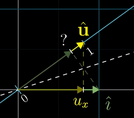
- In general, let’s imagine we have a number line that’s embedded in a 2-D space. Let $\hat{u}$ represent the vector that starts at the origin and ends on the number 1, on this number line. Thus, it is a unit vector.
- Assume we have a function that projects any 2-D vector onto this number line (this function goes from 2-D to a single real number). Think of this projection as a linear transformation. We aim to find the projection matrix that describes this projection function. Recall then that we need to find where the basis vectors $\hat{i}$ and $\hat{j}$ land on the number line after this projection/transformation.
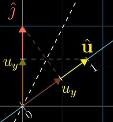
- From the following figure, you can see that the coordinate where $\hat{i}$ land on the number line, is simply $u_x$. Similarly, the coordinate where $\hat{j}$ land on the number line is simply $u_y$. Thus, we have the linear transformation matrix $[u_x, u_y]$, which transforms any vector in the original 2-D space onto the number line. Recall that the transformation we are talking about, is projecting any general vector onto the number line.
- Computing this projection transformation for any vector $[x, y]$ is computationally equivalent to taking the dot-product: \([u_x, u_y] \begin{bmatrix} x\\y \end{bmatrix} = u_x \cdot x + u_u \cdot y\)
- This is why taking the dot-product with the unit vector, can be interpreted as projecting a vector onto the span of the unit vector and noting the length.
- Summary: we had a linear transformation from 2-D space to the 1-D number line. Because this (projection) transformation is linear, it is described by some 1x2 matrix $[u_x, u_y]$. And matrix-vector product is numerically the same as dot-product: \([u_x, u_y] \begin{bmatrix} x\\y \end{bmatrix} = u_x \cdot x + u_y \cdot y\)
Eigenvector
- When performing a linear transformation, most vectors gets knocked off its original span (the line passing through the origin and the tip of the vector), ending up in a completely different direction and possibly a different length.
- However, there are some special vectors, called eigenvectors, that are quite unique. When these eigenvectors go through the transformation, they don’t change direction, they just get stretched or squished by a certain amount. This amount by which they stretch or squish is called the eigenvalue. Depending on the transformation, eigenvalue can be negative.
-
So, the eigenvectors (of the transformation) are like the “special” vectors that maintain their direction (stay on their span) and just get longer or shorter.
-
To understand what the transformation described by a matrix does, you can read off the columns of the matrix as the landing spots for the basis vectors. But, to understand what the transformation actually does (while being less dependent on the particular coordinate system), is to find the eigenvectors and eigenvalues.
- To find the eigenvectors and eigenvalues, you consider the equation $A \vec{v} = \lambda \vec{v}$. It’s like saying: For some special vectors $\vec{v}$, when I apply the transformation described by matrix $A$, it’s as if I just stretched or squished them by a factor of $\lambda$.
-
For instance, $(A - \lambda I)$ could be something like: \(\begin{bmatrix} 3-\lambda & 1 & 4\\ 1 & 5-\lambda & 9\\ 2 & 6 & 5-\lambda \end{bmatrix}\)
-
The only way for the product of a matrix $(A - \lambda I)$ with a non-zero vector $\vec{v}$ to become zero $(\vec{0})$, i.e. for the transformed vector to be the zero vector (transformation squashes or collapses the original vector $\vec{v}$ down to the origin), is if the transformation associated with the matrix squishes space into a lower dimension, i.e. $\text{det}(A - \lambda I)$ must be equal to 0. When you transform everything onto a line, the area of any region becomes 0.
PCA
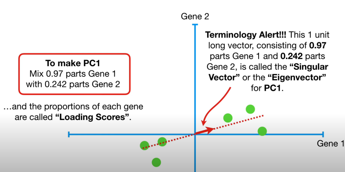
Given 2 variables, “Gene 1” and “Gene 2” and variables samples (green dots) instantiating these 2 variables, find the best fitting line (red dotted line).
- To find the best fitting line: Project each sample (dot) to the dotted line, then calculate disance of the projected point to the origin.
- To calculate distance of projected point to the origin, think of the dotted line as a transformation matrix; then do matrix-vector multiplication, then calculate L1-norm of resultant vector.
- Square each distance to the origin, then sum them up. The candidate line with the max sum-of-squares is the best fitting line (we call this PC1).
- We normalize this best fitting line, using the red arrow to indicate the unit vector $[0.97, 0.242]$ (0.97 represent the “gene-1” dimension, and 0.242 represent the “gene-2” dimension)
- This unit vector is called the “Singular vector” or “Eigenvector” for PC1.
- 0.97 (for gene-1) and 0.242 (for gene-2) are called the “loading scores”
- average of the sum-of-squares is called Eigenvalue for PC1: $\frac{\text{sum-of-square(distances for PC1})}{n-1} = \text{eigenvalue for PC1}$
- $\sqrt{\text{sum-of-square(distances for PC1)}} = \text{singular value for PC1}$
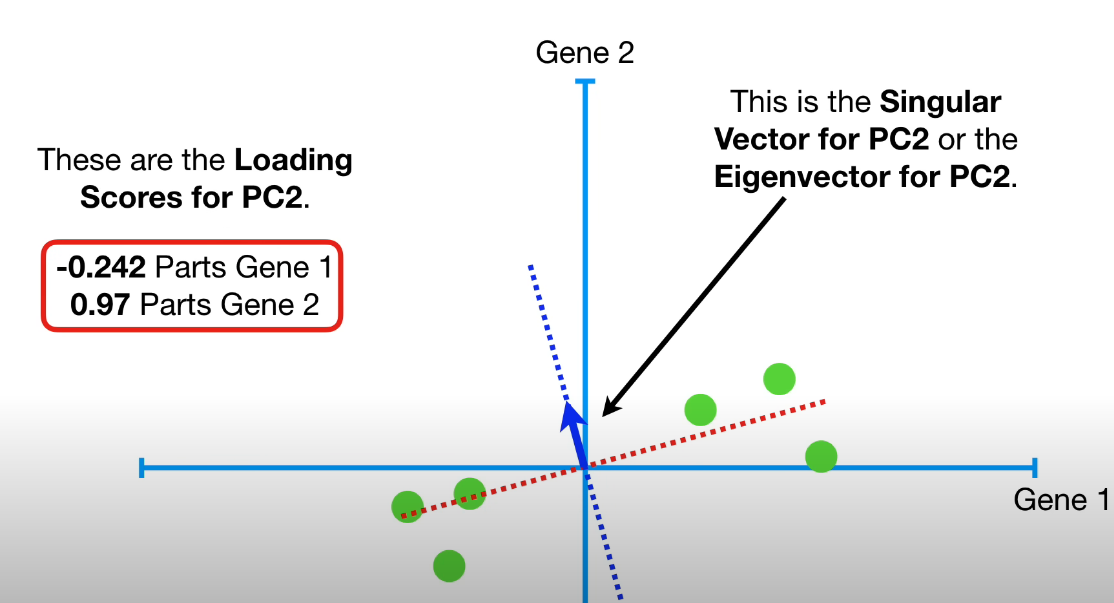
- To find PC2, it is the line through the orgin that is perpendicular to PC1.
- Unit vector for PC2 (aka singular vector/eigenvector for PC2) is represented by the blue arrow: $[-0.242, 0.97]$ (-0.242 parts gene-1, 0.97 parts gene-2)
- For PC2, gene-2 is 4 times as important as gene-1
- Unit vector for PC2 (aka singular vector/eigenvector for PC2) is represented by the blue arrow: $[-0.242, 0.97]$ (-0.242 parts gene-1, 0.97 parts gene-2)
- NOTE: Eigenvalues (average of the sum-of-square disances to the origin) are measures of variation
SVD
Given a $n \times m$ matrix $\mathbf{X}$, consisting of vectors $x_1, x_2, \ldots, x_m$, where each column $\vec{x} \in \mathbb{R}^{n}$ represent a data sample. SVD decomposes into:
- $\mathbf{U}$: $n \times n$ (left singular vectors) matrix. Consists of columns $u_1, u_2, \ldots, u_n$.
- These columns $\vec{u}$ are arranged from $1, \ldots, n$ in decreasing ability to describe the variance in the columns/data-samples of $\mathbf{X}$.
- This matrix is orthonormal, i.e. each $\vec{u}$ is a unit vector and these column vectors are orthogonal to one another. These column vectors provide a complete basis for the $n$ dimensions where $\mathbf{X}$ lives.
- $U U^{T} = U^{T} U = I$
- $\mathbf{\Sigma}$: $n \times m$ diagonal matrix.
- Each diagonal value $\sigma$ is non-negative and they are ordered such that $\sigma_{1} \ge \sigma_{2}$ and so on.
- Because of this ordering, ($u_1, v_1$) which corresponds to $\sigma_1$, are more important than ($u_2, v_2$) which corresponds to $\sigma_2$, and so on, in describing the information in $\mathbf{X}$. And the relative importance of each $u_k$ vs the other $\vec{u}$ are given by the relative values of the singular values $\sigma$ (and similarly for the vectors $v_k$)
- $\mathbf{V}^{T}$: $m \times m$ (right singular vectors) matrix.
- $V V^{T} = V^{T} V = I$
- The first column of $V^{T}$ will tell me the mixture that I can take on all the columns of $\mathbf{U}$, to add them up to equal $x_1$. So you can think of each column of $V^{T}$ as “mixtures” of the various $\vec{u}$ (scaled by $\sigma$) to make up each column vector $\vec{x}$
- $\mathbf{X} = \mathbf{U} \mathbf{\Sigma} \mathbf{V}^T = \sigma_{1} u_1 v_1^{T} + \sigma_{2} u_2 v_1^{T} + \ldots \sigma_{m} u_m v_m^{T}$. To see this:
- Note that the matrix $u_1 v_1^{T}$ is rank 1, because it has only 1 linearly independent column, and 1 linearly independent row.
- The sum: $\sigma_{1} u_1 v_1^{T} + \sigma_{2} u_2 v_1^{T} + \ldots \sigma_{m} u_m v_m^{T}$ increasingly improve the approximation of $\mathbf{X}$
We can think of the $\mathbf{U}$ and $\mathbf{V}$ matrices as eigenvectors of a correlation matrix given by $\mathbf{X} \mathbf{X}^T$ or $\mathbf{X}^{T} \mathbf{X}$. Why is $\mathbf{X}^{T} \mathbf{X}$ a correlation matrix? Observe:
- dim($\mathbf{X}^{T}$) = $m \times n$, dim($\mathbf{X}$) = $n \times m$
- Let $\mathbf{X}^{T}$ have rows $x_1^{T}, x_2^{T}, \ldots x_{m}^{T}$
- Let $\mathbf{X}$ have columns $x_1, x_2, \ldots x_{m}$
-
Then $\mathbf{X}^{T} \mathbf{X}$ = \(\begin{bmatrix} x_1^{T}x_1 & x_1^{T}x_2 & \ldots & x_1^{T}x_m \\ x_2^{T}x_1 & x_2^{T}x_2 & \ldots & x_2^{T}x_m \\ \vdots & \vdots & \cdots & \vdots \\ x_m^{T}x_1 & x_m^{T}x_2 & \ldots & x_m^{T} x_m\end{bmatrix}\)
- So this is a $m \times x$ matrix where each value is the $x_i \cdot x_j$ giving the similarity between $x_i$ and $x_j$.
- Notice that $\mathbf{X}^{T} \mathbf{X} = (\mathbf{U} \mathbf{\Sigma} \mathbf{V}^{T})^{T} \mathbf{U} \mathbf{\Sigma} \mathbf{V}^{T} = \mathbf{V} \mathbf{\Sigma} \mathbf{U}^{T} \mathbf{U} \mathbf{\Sigma} \mathbf{V}^{T} = \mathbf{V} \mathbf{\Sigma}^{2} \mathbf{V}^{T}$
- Multiplying both sides by $\mathbf{V}$ results in: $\mathbf{X}^{T} \mathbf{X} \mathbf{V} = \mathbf{V} \mathbf{\Sigma}^{2}$
- Hence, you see that $\mathbf{V}$ are the eigenvectors of the correlation matrix $\mathbf{X}^{T} \mathbf{X}$, while $\mathbf{\Sigma}$ is the square-root of its eigenvalues $\mathbf{\Sigma}^2$
- dim($\mathbf{X}^{T} \mathbf{X}$) = $m \times m$. You can think of this as correlation between data samples, so $\mathbf{V}$ represent the eigenvectors of the correlation between data samples.
- Notice that $\mathbf{X} \mathbf{X}^{T} = \mathbf{U} \mathbf{\Sigma} \mathbf{V}^{T} (\mathbf{V} \mathbf{\Sigma} \mathbf{U}^{T}) = \mathbf{U} \mathbf{\Sigma}^{2} \mathbf{U}^{T}$
- Multiplying both sides by $\mathbf{U}$ results in: $\mathbf{X} \mathbf{X}^{T} \mathbf{U} = \mathbf{U} \mathbf{\Sigma}^{2}$
- Hence, you see that $\mathbf{U}$ are the eigenvectors of the correlation matrix $\mathbf{X} \mathbf{X}^{T}$
- dim($\mathbf{X} \mathbf{X}^{T}$) = $n \times n$. You can think of this as correlation between features, so $\mathbf{U}$ represent the eigenvectors of the correlation between features.
