The ability to conduct efficient K-nearest neighbor (KNN) search is very important. Example applications are top-K web search results, clustering, etc. One technique for KNN is product quantization, which we discuss in this article. But first, some tibits of relevant information:

Norms

• L2 norm: Given a vector $\textbf{x} = [x_1, \ldots, x_n]$, its length ($L^2$ norm) is \(\| \textbf{x} \|_{2} = \sqrt{\sum_{i} x_{i}^{2}}\)

Computation Efficient Distance Calculation

• For distance between vectors $\textbf{x}$ and $\textbf{y}$, we can use Euclidean distance. For computation efficency, we often calculate the Squared Euclidean distance as \(\| \textbf{x} - \textbf{y} \|_{2}^{2} = \sum_{i} (x_i - y_i)^{2}\)
  • A naive implementation will loop through all dimensions $i$.
  • For computation efficiency, we can use matrix multiplication by simplifying $\sum_{i} (x_i - y_i)^2$ as follows: \((x_1 - y_1)^2 + \ldots + (x_n - y_n)^2 = x_1^2 + y_1^2 - 2 x_1 y_1 + \ldots + x_n^2 + y_n^2 - 2 x_n y_n\) \(= \textbf{x} \cdot \textbf{x} + \textbf{y} \cdot \textbf{y} - 2 (\textbf{x} \cdot \textbf{y})\) \(= \| \textbf{x} \|_{2}^{2} + \| \textbf{y} \|_{2}^{2} - 2(\textbf{x} \cdot \textbf{y})\)

Product Quantization

• To illustrate, here we assume each vector has 6 dimensions, which are divided into 3 chunks. We assume we have $\textbf{N}$ database vectors. To start off, we divide each database vector into 3 chunks of equal size.

Pre-Processing

• Run K-means separately for each chunk, i.e. here we will run 3 K-means.
  • The 1st K-means will cluster chunk-1 of all $\textbf{N}$ database vectors, clustering into $C=256$ clusters. Each cluster will have its own centriod. We repeat this for the 2nd K-means (clustering chunks-2 into $C$ clusters) and the 3rd K-means (clustering chunks-3 into $C$ clusters).
  • For each database vector, each of its chunks will be assigned to the nearest cluster. We represent this assignment with the cluster ID. Thus, we have now replaced with chunk in each database vector which was a list of Floats (each Float is 4 bytes), with a single Integer (1 byte). This compresses an original database vector $\textbf{x}$ into $\bar{\textbf{x}}$
• Within each chunk, create a pairwise distance map between all centriod pairs. With $C$ centriods, we produce $C \choose 2$ = $\frac{C (C-1)}{2}$ distance scores.

Decoding

• Given a test vector $\mathbf{x}$, we want to find the $K$-nearest database vectors.
  • Divide the test vector dimensions into 3 chunks. For chunk-1, calculate distance to all $C=256$ centriods associated with chunk-1. Repeat for chunk-2 and chunk-3. Let’s assume the test vector $\mathbf{x}$ has been compressed into $\bar{\mathbf{x}} = [c2, c123, c87]$
• Let’s assume that the first database vector $\mathbf{x}_1$ had been previously compressed into $\bar{\mathbf{x}}_1 = [c15, c80, c211]$. Using the previously calculated pairwise distance map, we calculate the distance of the test vector to this database vector: $\text{dist}(c2, c15) + \text{dist}(c123, c80) + \text{dist}(c87, c211)$. Repeat for all database vectors. Hence, distance computations to all $\mathbf{N}$ database vectors requires only $N*3$ lookups from the pre-computed distance maps.
• We now present the top-K database vectors that have the lowest summed distance.

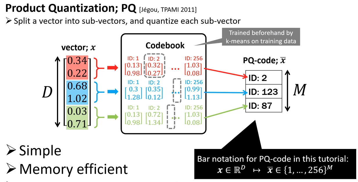Above image extracted from the CVPR20 tutorial by Yusuke Matsui.

Coarse Quantizer using Graph Traversal

For some problems, the search space is too large (too many database vectors). You can use Graph Traversal as a Coarse Quantizer, to first break down the search space into different regions. Then within each region, run Product Quantization.

Graph traversal

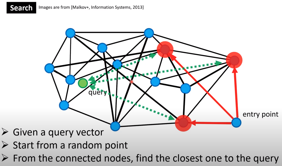
• The coarse quantizer is built using K-means.
• For a fast retrieval of KNN, we can use Graph Traversal.