Activation functions define the output of a node given its input. We describe here the Sigmoid, Tanh, ReLU, Leaky ReLU, ELU, and GELU.

Sigmoid (Logistic)

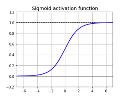
\(\sigma(x) = \frac{1}{1 + e^{-x}}\)

• Output range is positive from 0 to 1, centered at 0.5. Hence it is not zero-centered.
  • Hence even if our input is zero centered e.g. with values in (-1, 1), the activation layer will output all positive values. If the data coming into a neuron is always positive (i.e. $x_i \gt 0$ element-wise in $f = Wx + b$), the gradient of all the weights in $W$ will either be all $+$ or $-$, depending on the gradient of $f$ as a whole.
  • The above could introduce undesirable zig-zag movement in gradient updates, i.e. not a smooth path to the optimal.
  • This is partially resolved by using mini-batch gradient descent. Adding up across the batch of data, the weights updates could have variable signs.
• When inputs $-4 \lt x \lt 4$, the function saturates at 0 or 1, with a gradient very close to 0. This poses a vanishing gradient problem.
• Has an exponential operation, thus computational expensive.

Tanh

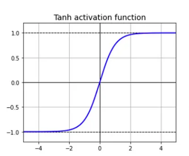
\(\text{tanh}(x) = \frac{e^x - e^{-x}}{e^x + e^{-x}}\)

• Output ranges from -1 to 1 and is zero-centered. This helps speed up convergence.
• When inputs become large or small around $-3 \lt x \lt 3$, the function saturates at -1 or 1, with gradient very close to 0.
• Has an exponential operation, thus computational expensive.

Rectified Linear Unit (ReLU)

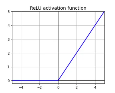
$f(x) = 0, \text{if } x \le 0$ OR, $f(x) = x, \text{if } x \gt 0$

• The gradient is 0 (for negative inputs), 1 (for positive inputs)
• The output does not have a maximum value.
• It is very fast to compute
• However, it suffers from dying ReLU. A neuron dies when its weights are such that the weighted sum of its inputs are negative for all instances in the training set. When this happens, ReLU outputs 0s, and gradient descent does not affect it anymore since when the input to ReLU is negative, its gradient is 0.

Leaky ReLU

\(f(x) = \text{max}(\alpha x, x)\)

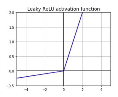
• Improvement over the ReLU. This will not have the dying ReLU problem. $\alpha$ is typically set to 0.01

Exponential Linear Unit (ELU)

\(f(x) = \alpha(e^{x} - 1), \text{ if } x \le 0 \text{, OR } f(x) = x, \text{ if } x \gt 0\)

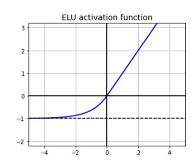
• This is a modification of Leaky ReLU. Instead of a straight line, ELU has a log curve for the negative values.
• Slower to compute than ReLU, due to exponential function. But has faster convergence rate.

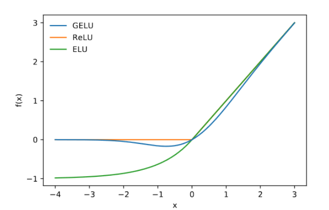
Gaussian Error Linear Unit (GELU)

GELU is used by BERT and GPT. The motivation behind GELU is to bridge stochastic regularizers (e.g. dropout) with activation functions.

• Dropout stochastically multiplies a neuron’s inputs with 0, thus randomly rendering neurons inactive. Activations such as ReLU multiplies inputs with 0 or 1, depending on the input’s value.
• GELU merges both, by multiplying inputs with a value $\phi(x)$ ranging from 0 to 1, and $\phi(x)$ depends on the input’s value.

\[\text{GELU}(x) = x \phi(x) = x P(X \le x), \text{ } X \sim N(0, 1)\]

As $x$ becomes smaller, $P(X \le x)$ corresponding becomes smaller, thus leading GELU to be more likely to drop a neuron, since $x P(X \le x)$ becomes smaller. So GELU is stochastic, but also depends on the input’s value.

• From the Figure, we see that $\text{GELU}(x)$ is 0 for small values of $x$.
• At around $x = -2$, $\text{GELU}(x)$ starts deviating from 0.
• When $x$ is positive, $P(X \le x)$ moves closer and closer to 1, thus $x P(X \le x)$ starts approximating $x$, i.e. approaches just $\text{ReLU}(x)$.

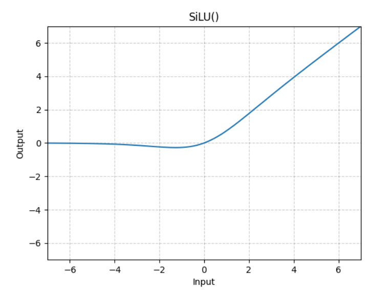
Swish-Gated Linear Unit (SwiGLU/SiLU)

When $\beta=1$, this is called the Sigmoid Linear Unit (SiLU) function: $\text{swish}(x) = x \text{ sigmoid } (\beta x) = \frac{x}{1 + e^{-\beta x}}$

The usual feed-forward layer in the transformer which uses ReLU is: $\text{max}(0, x W_1) W_2$.

LLaMA uses the Swish: \(\text{FFN}_{\text{SwiGLU}}(x, W, V, W_2) = (\text{Swish}_{\beta=1}(xW) \otimes xV) W_2\)

• $\otimes$ denote element wise multiplication
• dim($W$) = dim($V$) = dim $\times$ hidden_dim
• dim($W_2$) = hidden_dim $\times$ dim